|
|
|
Shelf-life prediction by microbial spoilage models rely on the assumption that relatively simple patterns of microbial growth and activity exist during food spoilage. It is well known that highly complex series of reactions take place during storage of food but many of these changes are not related to spoilage and shelf-life. For example, enzymatic and chemical reactions are usually responsible of the initial loss of freshness attributes whereas microbial activity is responsible for the overt spoilage and thereby determines product shelf-life (Dalgaard, 2000, Dalgaard 2003). Furthermore, food spoilage is dynamic with changes in spoilage reactions and changes between different groups of spoilage micro-organisms depending on product characteristics and storage conditions (Dalgaard 2000, Dalgaard 2006). This dynamic nature of food spoilage complicates the development of microbial spoilage models and the application of these models for shelf-life prediction. However, the concept of specific spoilage organisms (SSO) has allowed the formulation of microbial spoilage models (Dalgaard 2002). SSO has been defined as the part of the total micro-biota responsible for spoilage of a given product and the spoilage domain as the range of product characteristics and storage conditions within which a given SSO causes product rejection (Dalgaard, 1995). The graph below shows an example of the SSO-concept. As a consequence of the simple SSO-concept shelf-life can be predicted from:
|
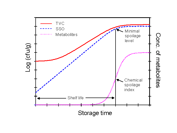 |
| Specific spoilage organism (SSO) concept. The minimal spoilage level and the chemical spoilage index are, respectively, the numbers of SSO and the concentration of metabolites determined at the time of sensory rejection (Dalgaard, 1993) |
|
Microbial spoilage models are typically developed by using a two step approach as shown in the figure just below: (i) A primary growth model is fitted to growth curve data to estimate the kinetic parameters e.g. maximum specific growth rate (Ámax), maximum cell concentration and lag time and (ii) a secondary model is then fitted to values for the relevant kinetic parameters. Often the effect of product characteristics and storage conditions on values of the maximum specific growth rare (Ámax) is the only secondary growth model needed. When microbial spoilage models are used to predict growth of microorganisms in food and thereby product shelf-life then the effect of product characteristics and storage conditions on kinetic parameters is determined first. Secondly, a predicted Ámax-value (and sometimes a lag time) is used together with a primary growth model to predict how the concentration of microorganisms change over time. |
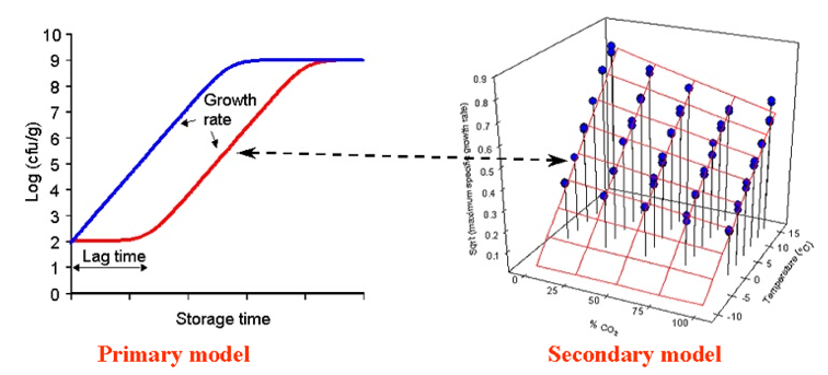
Figure modified from Dalgaard et al. (1997) with permission from Elsevier Ltd. |
| The microbial spoilage models in FSSP uses the log-transformed Logistic model as primary growth model and square-root or polynomial models as secondary growth models. See the different product specific MS-models in FSSP as well as Dalgaard (2002), Ross and Dalgaard (2004) and Dalaard (2009) for further details about primary and secondary growth models. |
| Microbial spoilage models must be evaluated in product validation studies
prior to use for shelf-life prediction. Accurate prediction of shelf-life
may be limited to specific foods or to a particular range of storage conditions.
Therefore, it is most important to determine the range of applicability for which a
microbial spoilage model is able to predicts shelf-life accurately enough for the model to be
useful in practice. The
range of applicability of microbial spoilage models depends very much on the range
of environmental factors for which a given SSO is responsible for spoilage of a food
i.e. the spoilage domain of the SSO. Microbial growth models can be evaluated by comparison of predictions with data from the literature or data from new experiments with naturally contaminated products. Observed and predicted data can be compared by graphical methods, indices of model performance like the bias- and accuracy- factors and by direct comparison of predicted and observed shelf-life. Clearly, comparison of the predicted shelf-life with shelf-life determined by a sensory panel is of outmost importance for microbial models developed from growth of a particular microorganism in a liquid laboratory medium. However, graphical methods and indices of model performance comparing observed and predicted lag times, maximum specific growth rates (Ámax) or times for a 1000-fold increase in cell concentrations can be useful. If, for example, a microbial model predicts a growth response that differs significantly from what is observed in food, then the model will also predict shelf-life incorrectly. Ross (1996) introduced the bias factor and the accuracy factor for evaluation of the performance of microbial growth models. The bias factor (Eqn. 1) indicates the systematic over- or under-prediction and with a value of e.g. 1.2 a model predicts growth 1.2 times (20%) faster than observed in food. In a similar way the accuracy factor (Eqn. 2) indicates the average deviation between observed and predicted growth. Recently, Mejlholm and Dalgaard (2013) suggested bias factor values for food spoilage micro-organism should be between 0.85 and 1.25 for a microbial spoilage model to be successfully validated. Previously, Dalgaard (2002) suggested that bias factor values for food spoilage micro-organism should be between 0.75 and 1.25 for a microbial spoilage model to be successfully validated. |
 Eqn.
1
Eqn.
1
|