|
|
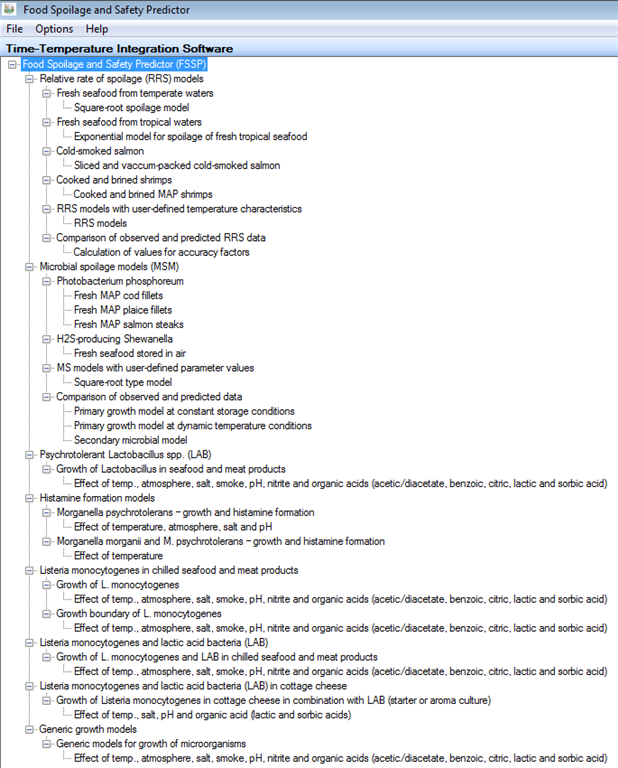
This section shows step-by-step how you can use the FSSP softwareModels and modules can be selected form the FSSP main window i.e. the thee-view structure shown below:
|
 |
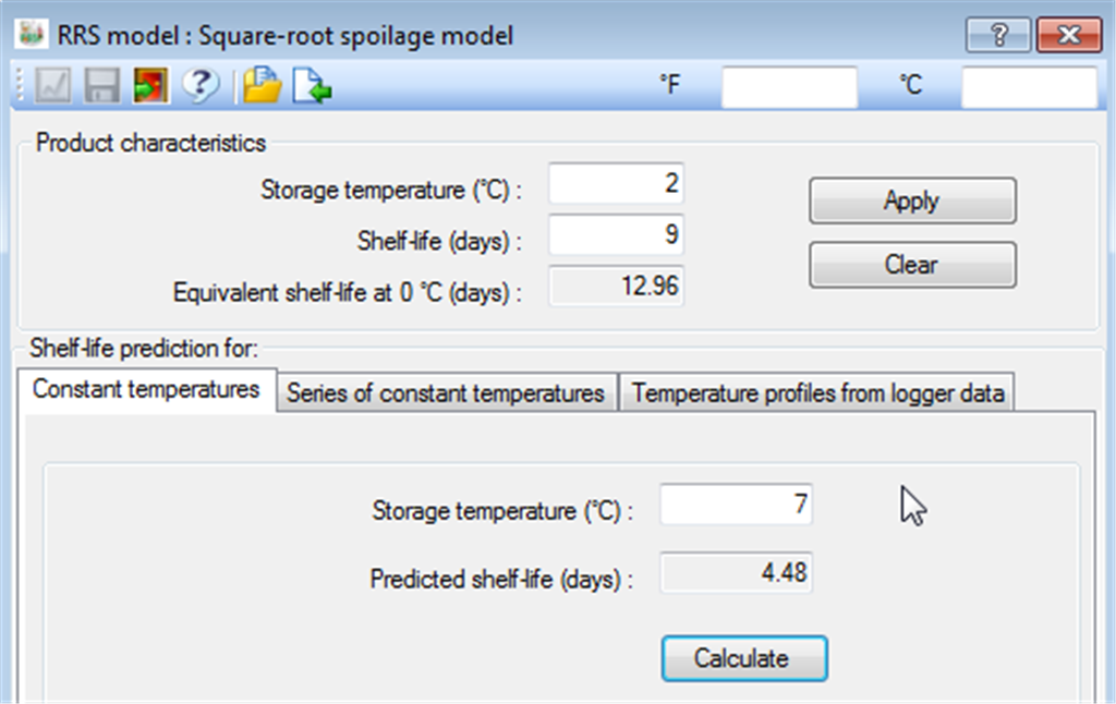
Relative rate of spoilage (RRS) models and general information about FSSP[FSSP home] Before any prediction can be performed product characteristics must be entered in the RRS model dialog box (as shown below). The only product characteristics required is the product shelf-life at a single known storage temperature (and then click on the APPLY button). From this information FSSP predicts shelf-life at different constant temperatures. To predict shelf-life in days, input a storage temperature in °C in the shelf-life prediction group-box and click on the CALCULATE button. Entering different constant temperatures is an easy way to get an idea about the temperature sensitivity of the product. In the dialog box shown below the shelf-life values are indicated with two decimals. However, from FSSP options (Options, General) the number of decimal places can be set by the user.
|
 |
Creating a temperature profile manuallyWithin the RRS-model dialog box and under the tab 'Series of constant
temperatures' (See picture just below) the storage temperature in °C and the
storage time in hours can be entered for each step of a temperature profile.
This is done by using the input fields as shown in the FSSP window below. Click on the
|
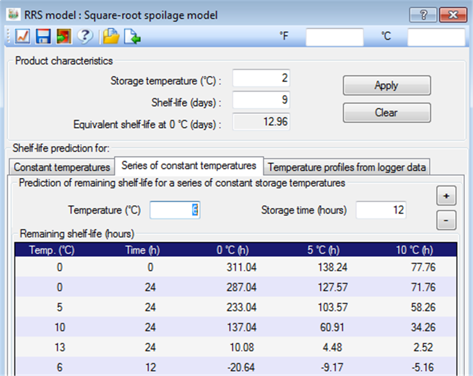 |
| You can include as many steps as you wish in a 'manual temperature profile'.
However, with more complicated profiles it is easier to generate a temperature
profile in a spreadsheet and to enter these data into FSSP as a ASCII file (See temperature
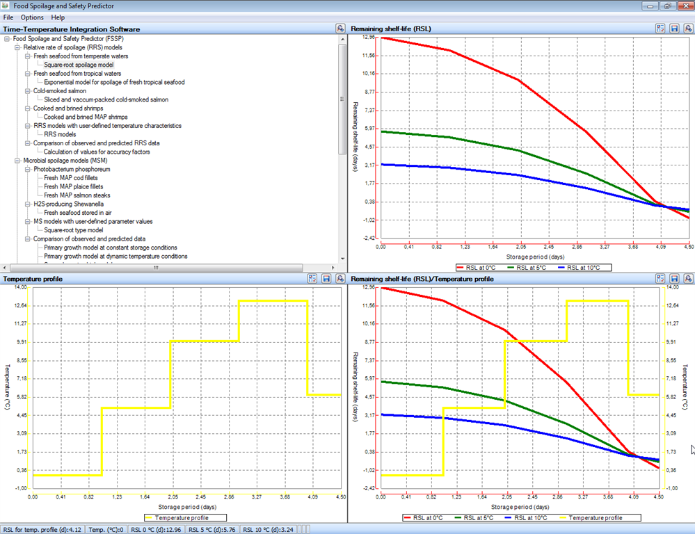
profiles) or by using the 'Raw data importer' ( To return from the FSSP output window with graphs (below) to the FSSP model dialog box (above) or to select a new FSSP model or module you need to double click on relevane model/module in the FSSP tree-view structure. |
 |
|
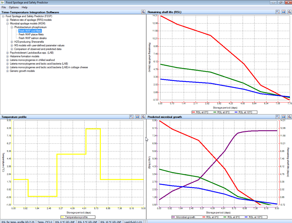
A results-bar is shown at the bottom of the FSSP output window just above. When FSSP users click on a curve by using the right mouse bottom this results-bar shows (i) remaining shelf-life (RSL) for the selected temperature profile, (ii) the actual storage temperature at that particular point in time and (iii) the remaining shelf-life (RSL) at 0°C, 5°C and 10°C. The remaining shelf life graph includes three curves showing the remaining shelf life at 0°C, 5°C and 10 °C. In each point in time the remaining shelf-life curves indicate remaining shelf-life of the product if stored at a constant temperature of 0°C, 5°C or 10°C until spoiled. Once a temperature profile has been entered in FSSP (manually, from an
ASCII file or by using the FSSP raw data importer) these data can be saved together with product characteristics in an
XML-file (Click on the
|
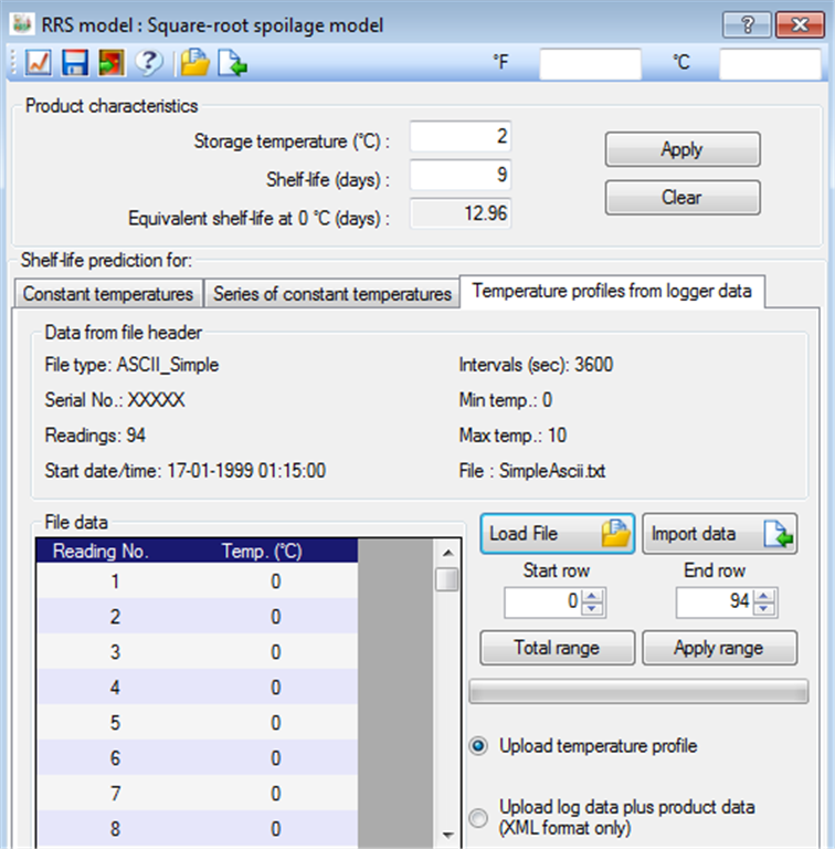
Entering temperature logger data into FSSPThe FSSP raw data importer (
|
 |
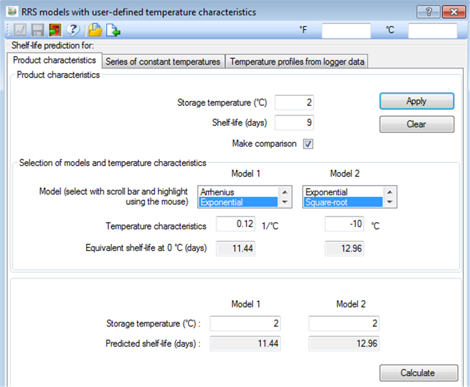
RRS models with user-defined temperature characteristicsIn addition to RRS models with fixed temperature characteristics corresponding to specific types of foods FSSP also includes RRS-models with user-defined temperature characteristics (See FSSP window below). These flexible RRS-models allow FSSP to predict shelf-life at different temperatures and for any food product where spoilage kinetics have been determined and the temperature characteristic is known to the user of FSSP. Users of FSSP can select (i) the Arrhenius-spoilage model and enter an apparent activation energy (Ea-value), (ii) the Exponential-spoilage model and enter a slope parameter value or (iii) the Square-root-spoilage model and enter a Tmin value. Two models can be selected at the same time to (a) compare two different temperature characteristics used with the same model or (b) to compare two different models with fixed temperature characteristics. Apart from their flexibility, the RRS-models with user-defined temperature characteristics function in the same way at the other RRS-models described above (See also Relative rate of spoilage (RRS) models).
|
 |
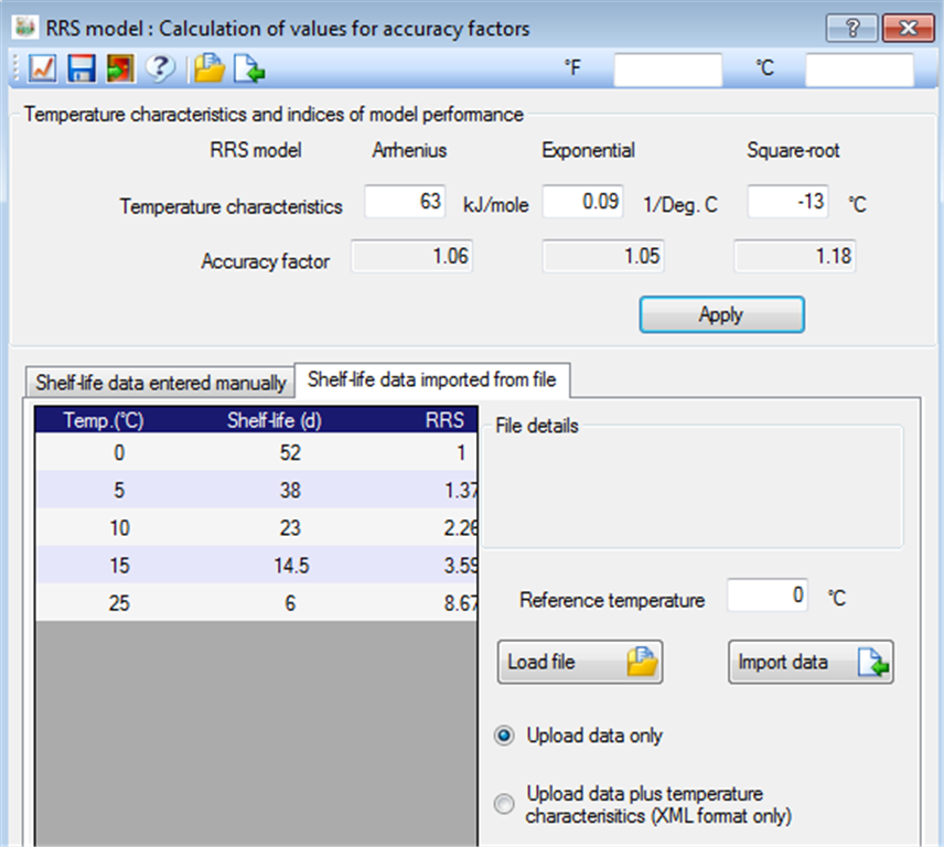
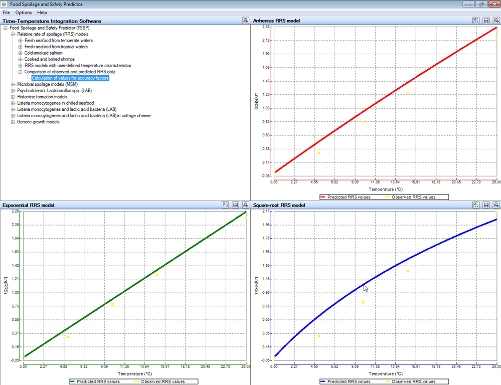
Comparison of observed and predicted RRS dataThis module of FSSP allows shelf-life data obtained at three different temperatures (or more) to be quantitatively compared with the Arrhenius, the Exponential or the Square-root spoilage models when used with a known temperature characteristic. Clearly, this includes any of the product specific RRS-models in FSSP. Thus, users can compare their own data with existing RRS-models in FSSP or evaluate if the Arrhenius, Exponential or Square-root spoilage models will be appropriate for their shelf-life data if these models are used with temperature characteristics optimal for the specific data. Shelf-life data can be entered manually as shown in the FSSP dialog box below.
Alternatively
data can be entered using the FSSP raw data importer ( FSSP uses relative rates of spoilage (RRS) to compare observed and predicted shelf-life data. The comparison rely on calculation of accuracy-factor values and presentation of observed and predicted data in graphs (See graphs in the FSSP output window below). When accuracy-factor values are calculated from RRS-data the reference temperature used to calulate RRS may influence the results. Therefore, FSSP determines average accuracy-factors. These average values are determined from the RRS data obtained by using all the tested storage temperatures as the reference temperature. |
 |
 |
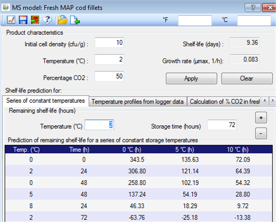
Microbial spoilage models (MSM)[FSSP home]. The MS-model dialog box is working in the same way as the RRS model dialog box described above. Predictions can only be performed after product characteristics have been entered. Product characteristics include (i) the initial concentration of bacteria in cfu/g (this value must be one or above), (ii) the storage temperature and (iii) possibly other factors like the level of carbon dioxide. When product characteristics have been entered, click on the APPLY button to calculate remaining shelf-life and microbial growth rate. By entering different sets of initial concentrations of bacteria (cfu/g) and storage conditions (temperatures or temperature and level of carbon dioxide) one can rapidly obtain an estimate of the products sensitivity with respect to 'the levels of contamination' and the storage conditions. The picture just below shows the MS-model dialog box in FSSP with calculated values. MS-models predict microbial growth and remaining shelf -life at constant or at
dynamic temperature storage conditions. Temperature profile data can be entered
as described above for the RRS-models. More information on this matter is found under temperature
profile data - FSSP formats. Click on the graph
icon in the upper left corner of the screen (
|
 |
 |
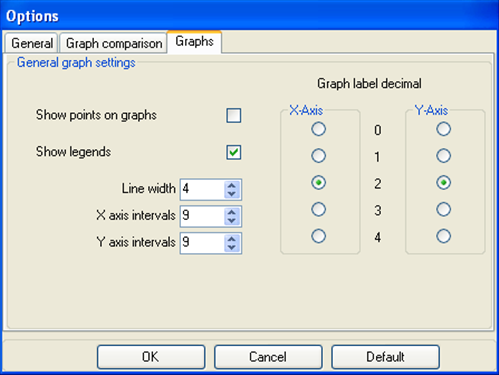
Options and zoom functions available in FSSP™ to modify graphs[FSSP home] FSSP includes several options
that allow the appearance of graphs to be modified by (i) changing
the width of lines/curves, (ii) changing the number intervals for tichmarks on
X- and Y-axis and (iii) including or excluding data points and
legends on graphs. OPTIONS are selected from individual gaphs (
|
 |
|
Depending on the type of model or module used, FSSP shows graphs of temperature profiles, remaining shelf-life, microbial growth (Log cfu/g) or microbial growth rate (1/h). Under OPTIONS, the GRAPH COMPARISON tab allows different overlay graphs to be produced. To focus on particular areas of graphs FSSP includes a zooming function. When graphs are visible the zooming function is activated by holding down the left mouse button and then moving the mouse to mark the area to be magnified. To revert the magnification click on the right mouse button. |